Python Analysis

The Python Analysis transform lets you write scripts using the Python programming language to perform statistical and predictive analysis on data or perform other data manipulation. This is similar to the Python Data Generator transform except that it operates on input data from a preceding transform instead of generating its own output.

To learn more about the Python language, see python.org.

1. Setup

The Python programming environment must be installed on the Dundas BI server for you to use the Python Analysis transform.

This is normally installed for you automatically as a prerequisite. See Install Python for more details, and for examples of how to install additional Python packages to use in your transforms.

2. Input

The Python Analysis transform requires one or more input transforms (each of which may produce multiple columns of data).

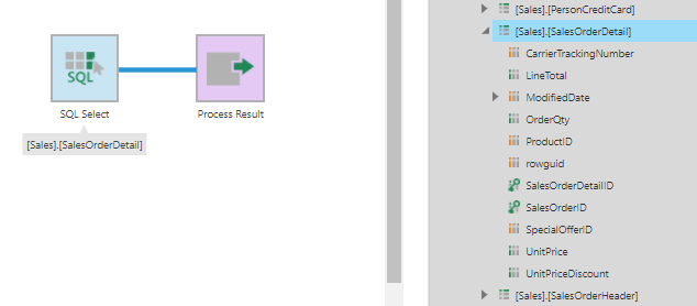
For example, the input could be a SQL Select transform that reads data from the AdventureWorks table [Sales].[SalesOrderDetail].

3. Add the transform

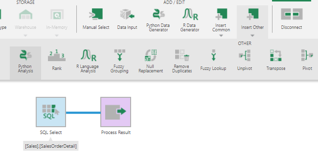
To add this transform to an existing data cube, first select the connection link between two connected transforms.

Go to the toolbar, click Insert Other, and then select Python Analysis.

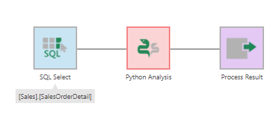
The Python Analysis transform is inserted between the two transforms and appears red because it needs further configuration.

4. Configure the transform

Double-click the Python Analysis transform (You can also select the Configure option from the context menu or the toolbar).

In the configuration dialog for the transform, the objective is to decide which input column(s) you want to analyze or apply processing to, and then enter a script that performs this analysis or processing on the input data.

For example, suppose you want to calculate the total sum of the OrderQty column from the input transform, and send this sum as the output.

To begin, click Define element placeholders in the configuration dialog. Click Add placeholder. In the Identifier text box, enter a variable name (for example, qty) for the input column which you will use in the Python script. Use the dropdown to select the corresponding input column (for example, OrderQty).

You can now write a Python script that references the qty variable by enclosing it between dollar sign characters. For example:

return sum($qty$)

This script calculates the sum of the OrderQty input column and returns the result as the output.

Select the Use Pooling option to reuse Python processes between execution of Python scripts to improve performance compared to starting a new process each time. There are corresponding configuration settings for Dundas BI administrators in the Python Pool category to manage the number of processes and their memory consumption.

5. Output

The output of the Python Analysis transform depends on the Python script it is configured with. It can be a single value, a column of values, or multiple columns.

6. Example Python script

The following example uses the polyfit function to find the least squares polynomial fit for the input columns.

6.1. Setup

This particular example relies on the NumPy package in Python and some input values:

• If the NumPy package is not installed, the Dundas BI server administrator can install it as described in the article Install Python.
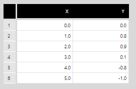
• For this example, in a new data cube, create a Data Input transform with the following two columns using the Double data type:
  • X: [0.0, 1.0, 2.0, 3.0, 4.0, 5.0]
  • Y: [0.0, 0.8, 0.9, 0.1, -0.8, -1.0]

  

6.2. Define placeholders

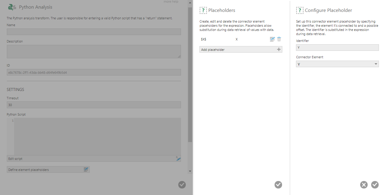
Add the Python Analysis transform and double-click to configure it. Click Define element placeholders, and then define the two placeholders X and Y.

6.3. Create the script

To fit the input values to a third-power polynomial, add the following script to the Python Analysis transform:

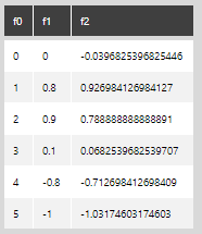
import numpy as np

Z = np.polyfit($X$, $Y$, 3)
P = np.poly1d(Z)

return ($X$, $Y$, P($X$))

The generated output is in the form of a table consisting of the X and Y inputs, as well as the polynomial values for each entry.

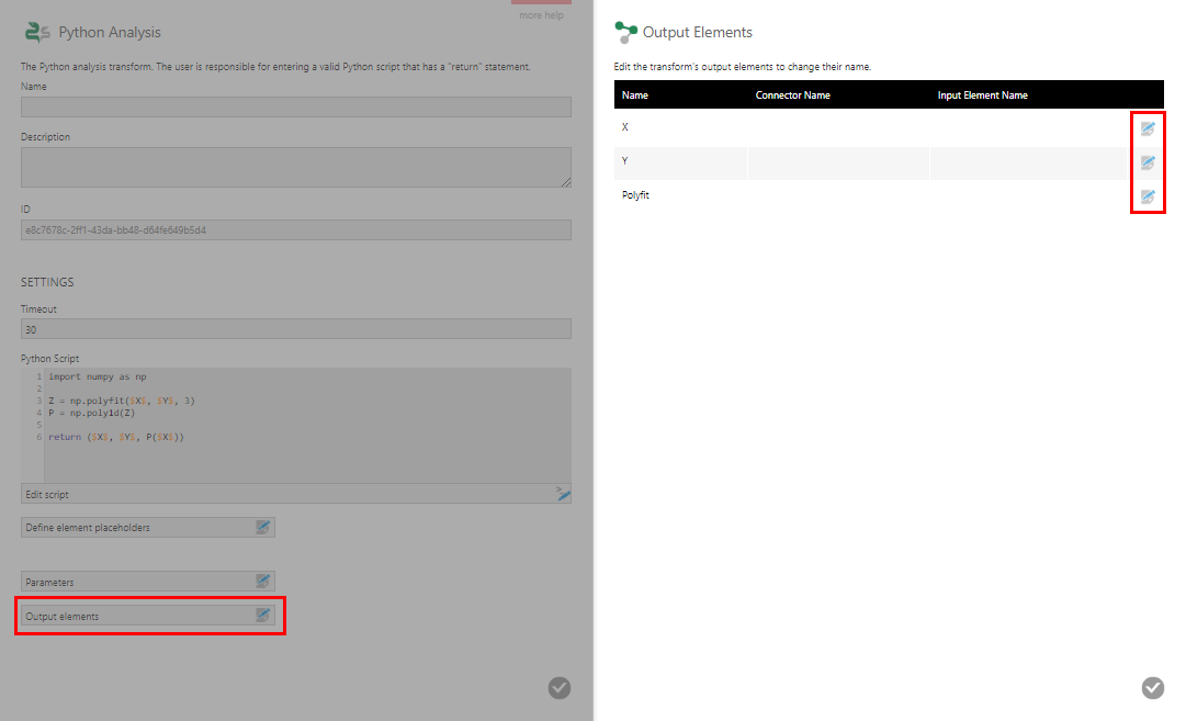
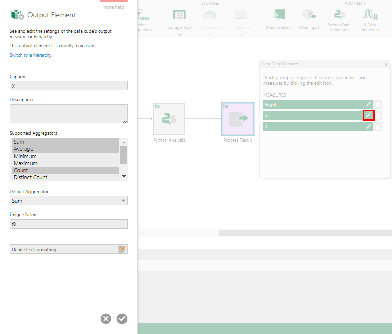
6.4. Adjust the column names and the output

Configure the transform again and click Edit output elements.

Edit each output element and provide a relevant column name.

Select the Process Result transform and edit the X measure. Click Switch to hierarchy and then select Count from the supported aggregators.

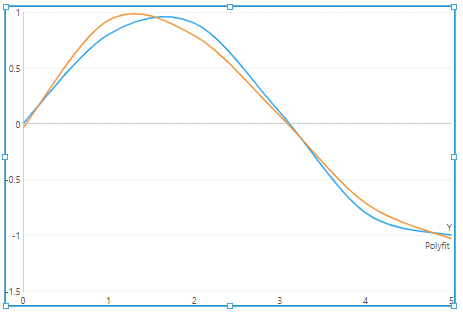
6.5. View the result

On a new dashboard, drag all three elements from the data cube and Re-Visualize as a Curved Line.

7. Geocoding addresses

A Python Analysis transform is one way you can convert street addresses in your data into latitude & longitude coordinates (also called 'geocoding'), which can then be plotted on a map visualization.

The following example uses the geopy package in Python to connect to the Mapbox geocoding service (using the 'temporary' geocoding API, meaning results are on-demand and not stored). The administrator of the Dundas BI server may need to install this package first, entering pip install geopy for example in a command prompt running as administrator.

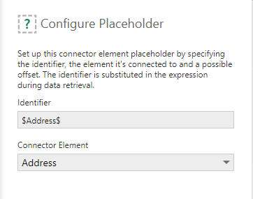
After adding a Python Analysis transform connected to your data source, click to configure it and click Define element placeholders. Add a placeholder with Identifier set to Address and Connector Element set to your address data.

You can also add other placeholders if you have other data you want to return and use in the transforms that follow this one.

Enter Python Script like the following. Edit the api_key value to your Mapbox access token, and edit the last line if you have additional placeholders you want to return:

import pandas
from geopy.geocoders import MapBox

geolocator = MapBox(api_key="<your MapBox API access token>")
locations = list(map(lambda address: geolocator.geocode(address), $Address$))

latitudes = list(map(lambda location: location.latitude if location != None else None, locations))
longitudes = list(map(lambda location: location.longitude if location != None else None, locations))

return pandas.DataFrame({"Address": $Address$, "Latitude": latitudes, "Longitude": longitudes})

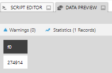
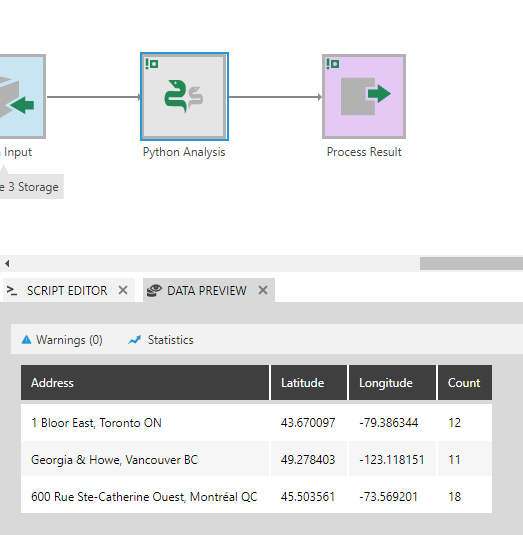
Your script will run when you submit the transform configuration dialog. You can expand Data Preview to view the output, including longitude and latitude coordinates:

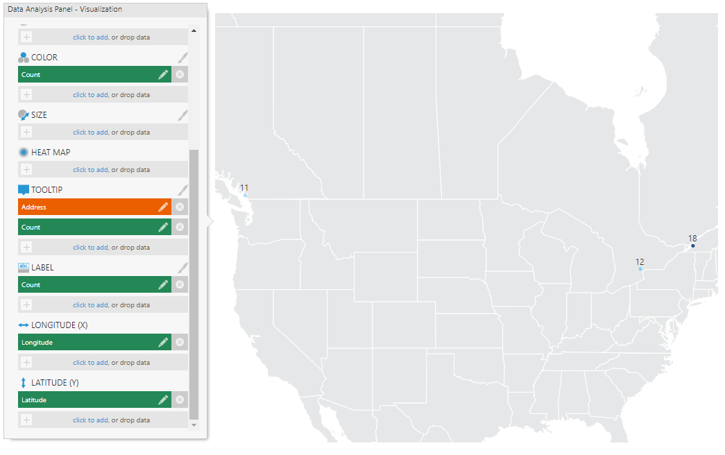
Now you can plot your addresses on a map using the steps shown in the article Displaying symbols on a map, using your data cube as the data source. You can start by dragging Address from your data cube in the Explore window onto a new metric set, for example, and re-visualizing to a Map.

In the Data Analysis Panel's Visualization tab, expand Symbols and assign the Longitude (X) and Latitude (Y) to the corresponding coordinates from your data, and assign other data to be visualized as you prefer.

Depending on your needs and how closely you are zoomed into your addresses, you can also set up the map to display street-level maps behind the symbols as context. Dundas BI maps support Mapbox static tiles as well as other map providers.

8. See also

• Install Python
• Transform: Python Data Generator
• Transform: R Language Analysis
• List of transforms
• Off the Charts: Adding Weather Data to Dundas BI is a Breeze
• Off the Charts: Advanced Sentiment Analysis in Dundas BI