
The complexity of work and problems that require unique solutions is ever-increasing, the growth and presence of data is astounding, and people like you are understandably demanding more and more from your analytics. Luckily for you, Dundas BI has made a habit of outpacing this mania, by continuously moving forward, maturing, and evolving. In fact, our relentless pursuit of perfection means that Dundas BI is constantly enriched with powerful new functionality to better guide users through their business intelligence and data analytics journeys and break down the barriers that prevent organizations from reacting, adjusting and tackling business priorities.
Today, I wanted to cover one such feature in Dundas BI that’s been newly released, which is the ability to perform more relevant period comparisons using a 13 Period Calendar. This is a type of calendar that consists of 13 periods of exactly 4 weeks each. It’s most often used for accounting purposes – but we recommend not limiting it to just that one use case – and is superior to the traditional 12-month calendar in that it offers better comparability of numbers between periods and assists in weekly report preparation by complementing a weekly cycle.
But before diving into that specific feature, I wanted to talk briefly about Time Dimensions, which set the stage for all time-based analysis in our software.
Introduction to time dimensions
To understand the role time dimensions play, we need to first understand how the Dundas BI Data Model is constructed. It is comprised of the following elements:
- Data Connectors
- Data Cubes (ETL)
- Hierarchies and Time Dimensions
- Metrics Sets
- Dashboards, Reports, Scorecards, and Small Multiples
A Hierarchy – commonly referred to as a Dimension – is used for grouping data into rows and columns and setting up drill downs. What’s great about hierarchies, is that they can be made up of one level, or of many levels, allowing users to easily drill up, down and into their data, expand upper-level items, and even change levels. A time dimension then, is simply a container for one or more Date or Time Hierarchies, that are based on the same calendar system.
There are many instances where a company would maintain data pertaining to the date and/or time some type of activity occurred, and a common one be in the case of the sale of an item or service. I’ve fabricated sales data for the sake of this exercise, to better explain how time dimensions work in Dundas BI. In this dataset we’ve two columns, a Sale_Value column, and a Date_Time column. The date_time column displays the date a specific sale occurred on, and the sale_value column displays the monetary value in dollars of that corresponding sale.
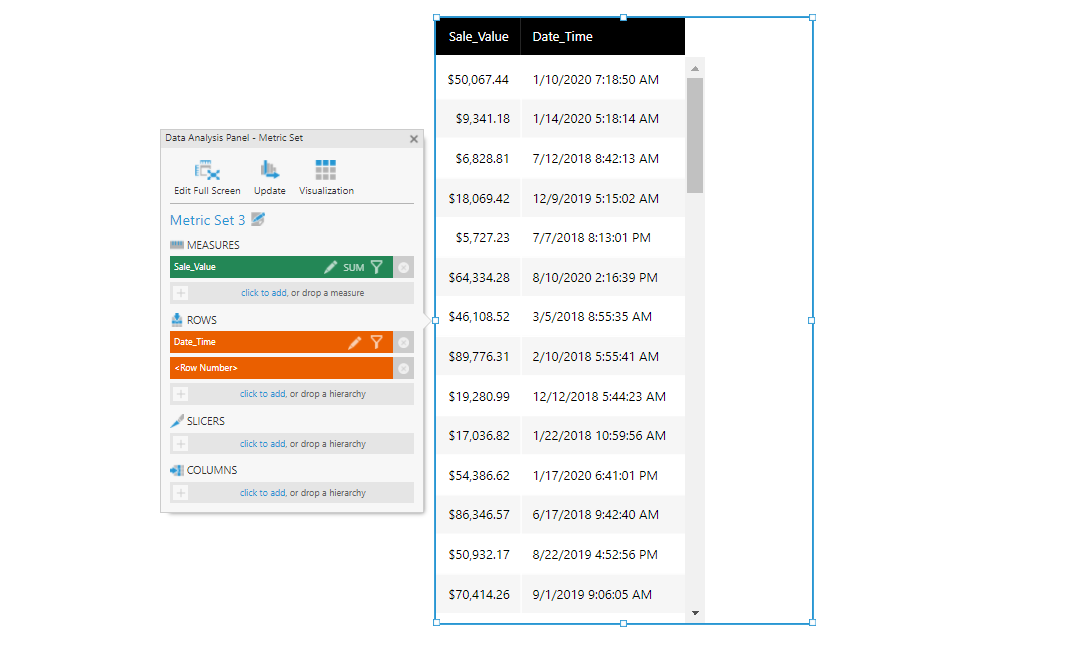
What you’re seeing in that image, is a laundry list of every sale that took place between October 1, 2017 and September 30, 2020. Included is the date, time, and monetary value of each transaction. You’ll notice that we’re showing raw SQL dates right now. There’s no order to those values, other than how we’ve ordered it in our database. With how it’s currently set up, we can’t perform any drills, and we can’t expand or group the data by any ‘like/same’ attributes – such as year, month, date, etc. When data is this raw, it’s not terribly useful.
Time dimensions now become critical if our goal is to perform time-based analysis. Without them, we wouldn’t be able to group or aggregate this data. So, this begs the question, how do we leverage time dimensions? Well, they’re easily accessible within Dundas BI; you simply need not look any further than the Explore Panel!
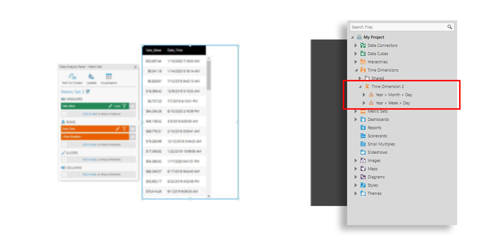
We can expand the time dimension folder, to unveil a few different time dimensions that are readily available within – such as Year > Month > Day and Year > Week > Day. Note that Dundas BI comes ready, out-of-the-box with a handful of time dimensions, but you’re also able to build your own. More on this later, when we talk about 13 Period Calendars.
Now, if we wanted to see one of these hierarchies in action, we simply need to drag it onto our Data Analysis Panel and drop it directly on top of our existing Date_Time row. Once we’ve done so, our visualization will automatically update and display our data using those aggregated groupings.
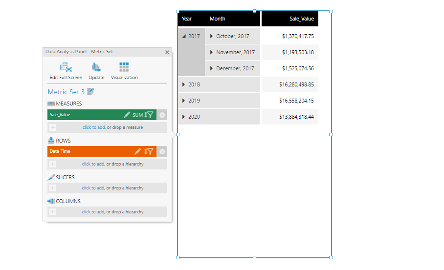
As you can see, I now have a succinct table with Year-level, Month-level, and Day-level drill downs automatically built into it, making it much easier to perform time-based analysis than with our raw data! This is the power of time dimensions in Dundas BI.
Building your own 13 period time dimension
The 13 period calendar is – as the name indicates – a calendar that is divided into 13 periods, where each period is exactly 4 weeks long – with a few exceptions. While the 12-month calendar is more common, there are in facts many arguments for the 13 period calendar. Holidays, for example, will occur in the same week of the same period every single year. If you compare this to a traditional calendar, you’ll find holidays often occur in different weeks across the years. Likewise, when using a 13 period calendar, the end of each period will always occur on the same day of the week, unlike with a 12-month calendar where month-ends can fall on any day of the week. There are other advantages beyond holidays as well. ‘Monthly’ comparisons, for example, can be more easily performed and are more relevant when using 13 identical 28-day periods. Since every period is consistent – i.e., contains the same number of weekdays and weekends – trends are also more accurate and easier to spot.
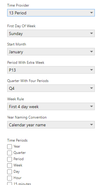
The following image displays which values you can define when creating 13 period calendars in Dundas BI. You’re able to set the Time Provider (i.e., calendar type), which day of the week your periods will begin on, which month will mark the start of your calendar, which period will contain an extra week – by nature, one period of a 13 period calendar will contain 5 weeks, where the other 12 will each contain 4 weeks – which quarter will contain an extra week – much like with periods, one quarter will contain an extra fourth period, the other 3 will each contain 3 periods – the week rule, the naming convention, and the time period cadence.
For more details on the types of time dimensions you can create using Dundas BI, I encourage you to check out this article on our Support Site.
Conclusion
Not every business begins its fiscal year in January or on the first of the month. Not every business reports on its data at the Year or Month levels; some are more interested in understanding what’s happening with their data in intervals of 5 or 10 minutes. And perhaps most importantly, not every business uses – or wants to use – Gregorian or Fiscal calendars.
With Dundas BI, we’re able to build our own time dimensions to reflect these nuances. If you’ve been looking for a way to report on your data using a 13 period structure, or if you’ve stumbled upon this and are now interested in doing so, you’re in luck. With Dundas BI, we’re able to build our own 13 period time dimension with just a few simple clicks and can perform more effective time-based analyses.
Follow Us
Support