So you or someone within your organization spent time to gather data, analyze it, choose a machine learning algorithm, train a model and you now finally hold the key to predict your future (at least from the data point of view). But what’s next? How can you take this machine learning model and integrate it with your BI platform so your prediction model can be used in your on-going decision making process in an automated fashion? In other words, how can you operationalize your model and apply it to new data coming through your applications like all other data analyzed through your BI system.
With Dundas BI, automating such a process is quite easy. Dundas BI’s rich data preparation layer allows you to leverage all the data connections you’ve already configured in the application, together with your favorite machine learning model created either in Python or R. The model is then executed as part of your data preparation process so the result can be used like any other dataset, leveraging the advanced visual layer of Dundas BI to share the insights with others. For example, you may have created a data connection to Google Analytics and have joined it together with data from your CRM system. Your data expert (data scientist/engineer), managed to create a machine learning model that is able to classify your customers based on your different data variables so you can then provide each customer group with services relevant to that group only. With Dundas BI’s built-in integration to Python and R, you can automatically classify (or score) each new customer that comes through your CRM and deliver the results to your dashboard consumers such as your customer success team. They can then better decide how to best engage with that customer according to the customer classification.
Ready to operationalize your predictive model? Read on for the implementation steps.
Implementation in Dundas BI
In most cases, a typical flow in machine learning involves using sample data called “training data” to train the predictive model to learn the known patterns within the sample dataset. This model is then used on unknown datasets to make predictions based on the trained model.
As mentioned above, using Dundas BI’s Python and R transforms, you can execute Python/R scripts that will call and load the pre-created machine learning model object and use it with new data using the following steps:
- Store your model object file created using Python/R in a place which is accessible to the Dundas BI server.
- Create a Data Cube in Dundas BI with the data you want queried and add to it a Python/R transform.
- Configure the Dundas BI Python/R data transform to use a Python/R script that loads the model object file and use it on the new data.
- The results will come back to the data flow of Dundas BI and the users can then use those with any other visual interactions in Dundas BI just like any other data.
Sample Implementation Using Python
The following example uses the popular Iris dataset and uses Google’s Tensorflow library that creates a Deep Neural Network classifier model that was trained using a training dataset to learn and identify the patterns of the Iris flowers species. This example is using Python but you can follow a similar process in R as well.
In order to train the model, training data is provided to the machine learning algorithm and the results are compared against a test dataset that contains known patterns (i.e. the actual species type of each Iris flower in our flowers samples). The model then learns and retrains how to identify the patterns and thus the species.
The model is then saved in an object file that is stored in a directory accessible to the Dundas BI server. Using Dundas BI’s Data Cube, this model is executed to identify the flower species in new data coming from another data source.
You can see this entire flow in action in our Predictive Analytics for Everyone webinar here (starting from 30:55).
Note you can download the related files used from here:
Download: Tensor Flow Iris Example
Follow the steps below to implement this on your end:
Train your model:
1. In your Python environment, open command prompt as the administrator, navigate to the C:\Program Files\Python36\Scripts folder and install tensorflow, numpy and pandas packages with the following command:
pip install tensorflow numpy pandas
2. Store the training and the test datasets at a location accessible to your Python environment. In this example, the datasets are located in the same folder as the iris_classifier.py file created below.
3. Create and train your deep neural network classifier model in Python and store the results in a directory. This example creates a model object file called iris_classifier.py using the relevant Google’s Tensorflow library.
import tensorflow as tf
import numpy as np
# Data sets
IRIS_TRAINING = "iris_training.csv"
IRIS_TEST = "iris_test.csv"
# Load datasets.
training_set = tf.contrib.learn.datasets.base.load_csv_with_header(filename=IRIS_TRAINING,
target_dtype=np.int,
features_dtype=np.float32,
target_column=-1)
test_set = tf.contrib.learn.datasets.base.load_csv_with_header(filename=IRIS_TEST,
target_dtype=np.int,
features_dtype=np.float32,
target_column=-1)
feature_columns = [tf.contrib.layers.real_valued_column("", dimension=1)]
# Build a 3 layer Deep Neural Network with 10, 20, 10 units respectively.
classifier = tf.contrib.learn.DNNClassifier(hidden_units=[10, 20, 10],
n_classes=3,
model_dir="c:/tfmodels/iris_model",
feature_columns=feature_columns)
# Fit model.
classifier.fit(x=training_set.data,
y=training_set.target,
steps=2000)
# Evaluate accuracy.
accuracy_score = classifier.evaluate(x=test_set.data,
y=test_set.target)["accuracy"]
print('Accuracy: {0:f}'.format(accuracy_score))
# Classify two new flower samples.
new_samples = np.array(
[[6.4, 3.2, 4.5, 1.5], [5.8, 3.1, 5.0, 1.7], [5.5,4.2,1.4,1.3]], dtype=float)
y = classifier.predict(new_samples)
print('Predictions: {}'.format(str(list(y))))
In order to run the model, navigate to the folder where iris_classifier.py file is located and execute it in the command line using:
python iris_classifier.py
There should now be a directory “c:/tfmodels/iris_model” created in the C: Drive.
Use the model in Dundas BI:
1. Ensure Python is installed on your Dundas BI server for all users.
2. In Dundas BI, create a data cube based on "Fisher's Iris Data.xlsx". You can exclude the species information from the dataset. We will use the trained classifier model created above to identify the species.
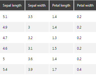
Figure 1: Iris dataset preview.
3. Add a Python Analysis transform and define the following placeholders to reference data inside the Python script that returns the results of the model in the next step.
Sepal length: $sepal_length$
Sepal width: $sepal_width$
Petal length: $petal_length$
Petal width: $petal_width$
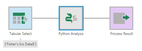
Figure 2: Add the Python transform.
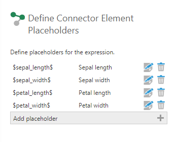
Figure 3: Define the placeholders.
4. Use the script below in the script editor of the Python transform to call the classifier model and feed the data into it to score new data. In other words, let the neural network identify the species of flowers and send it back to the data cube flow. The results are returned in a dataframe:
import tensorflow as tf
import numpy as np
import pandas as pd
feature_columns = [tf.contrib.layers.real_valued_column("", dimension=1)]
# Build a 3 layer Deep Neural Network with 10, 20, 10 units respectively.
classifier = tf.contrib.learn.DNNClassifier(hidden_units=[10, 20, 10],
n_classes=3,
model_dir="c:/tfmodels/iris_model",
feature_columns=feature_columns)
samples = np.array(list(map(list,zip($sepal_length$, $sepal_width$, $petal_length$, $petal_width$))), dtype=float)
result_column = list(classifier.predict(samples))
speciesList = ["I. setosa", "I. versicolor", "I. virginica"]
species = list(map(lambda speciesId: speciesList[speciesId], result_column))
result = pd.DataFrame(data = {
"Sepal length": $sepal_length$,
"Sepal width": $sepal_width$,
"Petal length": $petal_length$,
"Petal width": $petal_width$,
"Species": species
})
return result
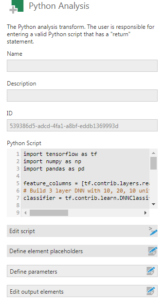
Figure 4: Implement the script in the Script Editor.
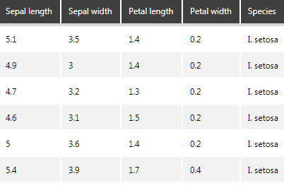
Figure 5: Result of the Python transform.
5. To avoid unnecessary aggregation, add a Rank transform. Select any element as the sorting element, and ensure that the ranking method is set to "Standard". Name the output "SampleId" and make sure to switch it to a hierarchy under the process result transform.

Figure 6: Add the Rank transform.
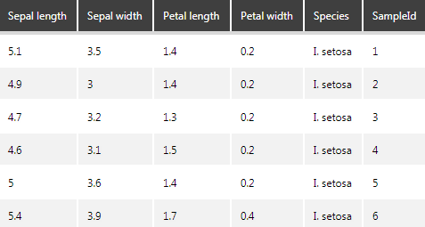
Figure 7: Result of the Rank transform.
Visualize the result
Now that you have the result, you can create metric sets and visualize them. For example, the above result can be visualized into a point chart with the colors demarcating the clusters as shown below:
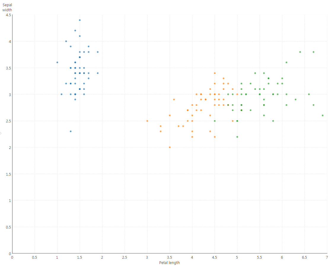
Figure 8: Visualize the results in a Scatter plot.
To get this result, create a Metric Set, and from the data cube created above, add the following on the Data Analysis Panel:
Measures: Sepal Width and Petal Length
Rows: SampleId and Species
Color: Species
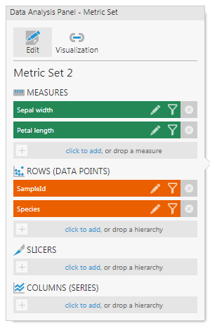
Figure 9: Data Analysis panel for the Scatter Plot.
Conclusion
If you already went through the heavy lifting of creating a predictive model, automating the usage of it is just a few steps away when using Dundas BI. The benefit will be in your ability to go beyond descriptive or diagnostic analytics, by gaining predictive analytics capabilities all within the same enterprise BI solution already connected to your data and used by all users for all other BI use cases. You can even take it to the next level and turn it into a fully prescriptive analytics model by visualizing a recommendation or integrating it with other services that can automate a full action.


Follow Us
Support